Modeling risk with covariates
Set up
Section titled “Set up”import matplotlib.pyplot as pltimport numpy as npimport polars as pl
import tausurv as tsfrom tausurv.step import StepFunction
%config InlineBackend.figure_format = 'svg'
ts.plot.set_style("publication")Looking at the cohort with polars
Section titled “Looking at the cohort with polars”ts.datasets.load_pbc returns a SurvivalBunch that tuple-unpacks as (X, Y, delta), with the covariates in a polars DataFrame.
pbc = ts.datasets.load_pbc()X, Y, delta = pbcY = Y / 365.25
X.head()
shape: (5, 17) ┌─────┬───────────┬─────┬─────────┬───┬──────┬──────────┬─────────┬───────┐ │ trt ┆ age ┆ sex ┆ ascites ┆ … ┆ trig ┆ platelet ┆ protime ┆ stage │ │ --- ┆ --- ┆ --- ┆ --- ┆ ┆ --- ┆ --- ┆ --- ┆ --- │ │ i64 ┆ f64 ┆ str ┆ i64 ┆ ┆ i64 ┆ i64 ┆ f64 ┆ i64 │ ╞═════╪═══════════╪═════╪═════════╪═══╪══════╪══════════╪═════════╪═══════╡ │ 1 ┆ 58.765229 ┆ f ┆ 1 ┆ … ┆ 172 ┆ 190 ┆ 12.2 ┆ 4 │ │ 1 ┆ 56.44627 ┆ f ┆ 0 ┆ … ┆ 88 ┆ 221 ┆ 10.6 ┆ 3 │ │ 1 ┆ 70.072553 ┆ m ┆ 0 ┆ … ┆ 55 ┆ 151 ┆ 12.0 ┆ 4 │ │ 1 ┆ 54.740589 ┆ f ┆ 0 ┆ … ┆ 92 ┆ 183 ┆ 10.3 ┆ 4 │ │ 2 ┆ 38.105407 ┆ f ┆ 0 ┆ … ┆ 72 ┆ 136 ┆ 10.9 ┆ 3 │ └─────┴───────────┴─────┴─────────┴───┴──────┴──────────┴─────────┴───────┘
Seventeen covariates, mostly numeric, a few categorical (sex, edema). Some columns have missing values; null_count reports the per-column count.
X.null_count()shape: (1, 17) ┌─────┬─────┬─────┬─────────┬───┬──────┬──────────┬─────────┬───────┐ │ trt ┆ age ┆ sex ┆ ascites ┆ … ┆ trig ┆ platelet ┆ protime ┆ stage │ │ --- ┆ --- ┆ --- ┆ --- ┆ ┆ --- ┆ --- ┆ --- ┆ --- │ │ u32 ┆ u32 ┆ u32 ┆ u32 ┆ ┆ u32 ┆ u32 ┆ u32 ┆ u32 │ ╞═════╪═════╪═════╪═════════╪═══╪══════╪══════════╪═════════╪═══════╡ │ 106 ┆ 0 ┆ 0 ┆ 106 ┆ … ┆ 136 ┆ 11 ┆ 2 ┆ 6 │ └─────┴─────┴─────┴─────────┴───┴──────┴──────────┴─────────┴───────┘
Treatment arm (trt) is missing for the 106 non-randomised follow-up patients. Several lab measurements (chol, copper, alk.phos, ast, trig, platelet, protime) are missing for a handful of patients. The model uses five covariates that are clinically important and rarely missing: age, sex, stage (histologic stage), bili (bilirubin, mg/dL) and albumin (g/dL).
keep = ["age", "sex", "stage", "bili", "albumin"]X.select(keep).describe()shape: (9, 6) ┌────────────┬───────────┬──────┬──────────┬──────────┬──────────┐ │ statistic ┆ age ┆ sex ┆ stage ┆ bili ┆ albumin │ │ --- ┆ --- ┆ --- ┆ --- ┆ --- ┆ --- │ │ str ┆ f64 ┆ str ┆ f64 ┆ f64 ┆ f64 │ ╞════════════╪═══════════╪══════╪══════════╪══════════╪══════════╡ │ count ┆ 418.0 ┆ 418 ┆ 412.0 ┆ 418.0 ┆ 418.0 │ │ null_count ┆ 0.0 ┆ 0 ┆ 6.0 ┆ 0.0 ┆ 0.0 │ │ mean ┆ 50.741551 ┆ null ┆ 3.024272 ┆ 3.220813 ┆ 3.49744 │ │ std ┆ 10.447214 ┆ null ┆ 0.882042 ┆ 4.407506 ┆ 0.424972 │ │ min ┆ 26.277892 ┆ f ┆ 1.0 ┆ 0.3 ┆ 1.96 │ │ 25% ┆ 42.787132 ┆ null ┆ 2.0 ┆ 0.8 ┆ 3.24 │ │ 50% ┆ 51.000684 ┆ null ┆ 3.0 ┆ 1.4 ┆ 3.53 │ │ 75% ┆ 58.264203 ┆ null ┆ 4.0 ┆ 3.4 ┆ 3.77 │ │ max ┆ 78.439425 ┆ m ┆ 4.0 ┆ 28.0 ┆ 4.64 │ └────────────┴───────────┴──────┴──────────┴──────────┴──────────┘
Preparing the covariates
Section titled “Preparing the covariates”Select the five columns with their row index, drop rows with a missing value, encode sex as a 0/1 indicator and convert to NumPy. The row index subsets Y and delta to the same rows.
df = pbc.X.select(keep).with_row_index("_row").drop_nulls()kept_rows = df["_row"].to_numpy()df = (    df.drop("_row")    .with_columns(        sex_male=(pl.col("sex") == "m").cast(pl.Int8),    )    .drop("sex")    .select(["age", "stage", "bili", "albumin", "sex_male"]))
X_array = df.to_numpy().astype(np.float64)Y_kept = Y[kept_rows]delta_kept = delta[kept_rows]feature_names = list(df.columns)
print(f"{len(Y_kept)} patients kept ({len(Y) - len(Y_kept)} dropped for missingness)")
412 patients kept (6 dropped for missingness)
A 70/30 train/test split keeps patients aside for evaluation. With 412 patients the test set is small, so the evaluation scores below are imprecise.
rng = np.random.default_rng(seed=42)order = rng.permutation(len(Y_kept))split = int(0.7 * len(Y_kept))train, test = order[:split], order[split:]
X_train, Y_train, d_train = X_array[train], Y_kept[train], delta_kept[train]X_test, Y_test, d_test = X_array[test], Y_kept[test], delta_kept[test]
print(    f"train: n = {len(Y_train)}, events = {int(d_train.sum())}    "    f"test: n = {len(Y_test)}, events = {int(d_test.sum())}")
train: n = 288, events = 109 test: n = 124, events = 48
Fit the Cox model
Section titled “Fit the Cox model”The Cox model parameterises the hazard as and estimates by maximising Cox’s partial likelihood. ts.linear.CoxPH takes the design matrix and the observed-time / event-indicator arrays and returns a fitted estimator carrying coef_ (the ) and a baseline cumulative hazard.
cox = ts.linear.CoxPH().fit(X_train, Y_train, d_train)Reading the coefficients
Section titled “Reading the coefficients”Hazard ratios are read on the scale of the hazard, log-hazard coefficients are not. The table lists both; the forest plot shows the hazard ratios with confidence intervals.
coefs = pl.DataFrame( { "covariate": feature_names, "coef": cox.coef_, "HR": np.exp(cox.coef_), }).sort("HR", descending=True)coefsshape: (5, 3) ┌───────────┬───────────┬──────────┐ │ covariate ┆ coef ┆ HR │ │ --- ┆ --- ┆ --- │ │ str ┆ f64 ┆ f64 │ ╞═══════════╪═══════════╪══════════╡ │ stage ┆ 0.455048 ┆ 1.57625 │ │ sex_male ┆ 0.32355 ┆ 1.382025 │ │ bili ┆ 0.133439 ┆ 1.142752 │ │ age ┆ 0.027324 ┆ 1.0277 │ │ albumin ┆ -1.058192 ┆ 0.347083 │ └───────────┴───────────┴──────────┘
ts.plot.forest( names=feature_names, estimates=np.exp(cox.coef_), ci=np.exp(cox.confidence_intervals()), xlabel="Hazard ratio (per 1-unit increase)",)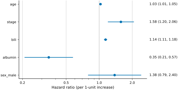
Holding the other covariates fixed, each step up in histologic stage multiplies the hazard of death by 1.58, each additional mg/dL of bilirubin by 1.14 and each year of age by 1.03; male sex has a hazard ratio of 1.38. Albumin is the one protective covariate: each additional g/dL multiplies the hazard by 0.35, consistent with albumin as a marker of preserved liver function. Hazard ratios per unit are not comparable across covariates measured in different units.
The bars are Wald 95% intervals from the inverse observed information at , exponentiated onto the hazard-ratio scale.
What the model says about specific patients
Section titled “What the model says about specific patients”Once and are known the model can produce a full survival curve for any covariate profile through . We contrast two illustrative profiles: an early-stage patient with normal labs and a late-stage patient with markedly abnormal labs.
profiles = {    "Early PBC, age 50, normal labs": np.array(        [50.0, 1.0, 0.6, 4.0, 0.0]  # age, stage, bili, albumin, sex_male    ),    "Advanced PBC, age 70, abnormal labs": np.array([70.0, 4.0, 8.0, 2.8, 0.0]),}
times_grid = np.linspace(0.1, 12.0, 240)S_profiles = cox.predict_survival_function(    np.stack(list(profiles.values())), times_grid)
fig, ax = plt.subplots()for label, s in zip(profiles, S_profiles, strict=True):    S_obj = StepFunction(time=times_grid, value=s, baseline=1.0)    ts.plot.km(S_obj, ax=ax, label=label)ax.set_xlabel("years from registration")
Text(0.5, 0, ‘years from registration’)
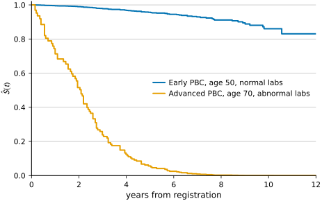
The early-stage profile keeps a predicted survival of 0.83 at twelve years. The advanced profile falls to 0.51 at two years and 0.05 at five.
Why is the advanced profile so high-risk?
Section titled “Why is the advanced profile so high-risk?”A hazard ratio is a per-unit effect and does not say which covariates account for the gap between one patient’s predicted survival and that of a reference patient. SurvSHAP(t) (Krzyzinski et al. 2023) splits that gap into one contribution per covariate at each time. With five covariates, the exact Shapley values take predictions.
from itertools import combinations, productfrom math import factorial
times_shap = np.linspace(0.1, 12.0, 100)x_ref = X_train.mean(axis=0)x_target = profiles["Advanced PBC, age 70, abnormal labs"]d = len(x_target)
# Precompute $S(t \mid x)$ for every one of the $2^d = 32$ feature-subset# assignments in a single batched call. ``masks[i, j] = 1`` means feature# ``j`` takes the target's value in row ``i``; ``0`` means it takes the# cohort-mean reference.masks = np.array(list(product([0, 1], repeat=d)), dtype=bool)X_subsets = np.where(masks, x_target, x_ref)S_subsets = cox.predict_survival_function(X_subsets, times_shap)mask_row = {frozenset(np.where(m)[0]): i for i, m in enumerate(masks)}
S_baseline = S_subsets[mask_row[frozenset()]]
shap_vals = np.zeros((d, len(times_shap)))for j in range(d):    others = [k for k in range(d) if k != j]    for k in range(d):        for subset in combinations(others, k):            weight = factorial(k) * factorial(d - k - 1) / factorial(d)            shap_vals[j] += weight * (                S_subsets[mask_row[frozenset(list(subset) + [j])]]                - S_subsets[mask_row[frozenset(subset)]]            )
ts.plot.shap.local_decomposition(    shap_vals,    baseline_survival=S_baseline,    times=times_shap,    features=feature_names,    xlabel="years from registration",)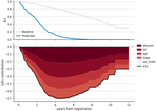
The top panel shows the predicted survival of a reference patient with the training-set mean covariates (dashed) and of the advanced profile (solid); the vertical gap between them is the sum of the SHAP values. The bottom panel splits that gap by covariate, with positive contributions stacked upward from zero and negative ones downward.
All four clinical covariates lower the advanced profile’s survival, most strongly at about 4.5 years. Albumin contributes most (up to 0.22 in survival probability; 2.8 g/dL against a mean of 3.5), followed by bilirubin (0.20), age (0.16) and stage (0.14); sex contributes almost nothing (0.01), since both the profile and most of the cohort are female. For more covariates or a nonlinear model, compute the SHAP array with another explainer (shap, survshap) and pass it to the same plot.
Across the cohort: which features matter when?
Section titled “Across the cohort: which features matter when?”The same computation for every training patient shows which covariates matter across the cohort and at which times. The code predicts survival under each of the 32 covariate subsets once for the whole training set, then combines the predictions as above.
subset_S = {}for k in range(d + 1):    for subset in combinations(range(d), k):        X_mod = X_train.copy()        not_in = [j for j in range(d) if j not in subset]        X_mod[:, not_in] = x_ref[not_in]        subset_S[frozenset(subset)] = cox.predict_survival_function(X_mod, times_shap)
shap_cohort = np.zeros((len(X_train), d, len(times_shap)))for j in range(d):    others = [m for m in range(d) if m != j]    for k in range(d):        for subset in combinations(others, k):            weight = factorial(k) * factorial(d - k - 1) / factorial(d)            shap_cohort[:, j, :] += weight * (                subset_S[frozenset(list(subset) + [j])] - subset_S[frozenset(subset)]            )
ts.plot.shap.feature_time_heatmap(    shap_cohort,    times=times_shap,    features=feature_names,    xlabel="years from registration",)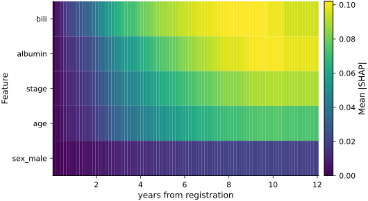
Rows are covariates, columns are times, and each cell is the mean absolute SHAP value over training patients. Bilirubin and albumin carry the most attribution (maximum mean absolute value 0.10 each), followed by stage (0.09) and age (0.07), with sex far behind (0.02). Attribution grows with time and peaks at nine to ten years for every covariate, later than for the single advanced profile, whose predicted survival is near zero by then.
How well does the model fit?
Section titled “How well does the model fit?”Calibration at a fixed time checks whether predicted survival probabilities agree with observed survival within groups of similar predictions. The Brier score at each time measures discrimination and calibration together; a perfect prediction scores zero.
eval_grid = np.linspace(0.1, 12.0, 200)S_test = cox.predict_survival_function(X_test, eval_grid)
predicted_5y, observed_5y, _ = ts.metrics.calibration.curve(    Y_test,    d_test,    S_test,    eval_grid,    t=5.0,    n_bins=5,)
ts.plot.calibration(    predicted_5y,    observed_5y,    xlabel="Predicted 5-year survival",    ylabel="Observed 5-year survival (KM in bin)",)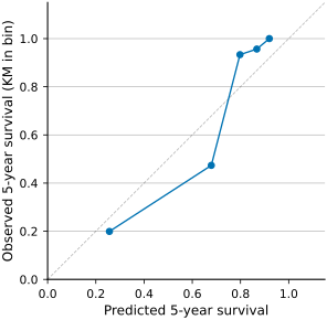
Each point is one of five quantile bins of predicted five-year survival; its x-coordinate is the bin’s mean prediction and its y-coordinate is the Kaplan-Meier estimate of survival at five years among the bin’s test patients. A perfectly calibrated model would have all points on the dashed identity line.
One test split gives one noisy estimate of the Brier score at each time. Five-fold cross-validation fits the model on 80% of the patients and scores the remaining 20%, five times, giving five estimates per time. Passing the resulting (n_folds, n_horizons) matrix to ts.plot.brier_over_time as values draws the mean as the line and a standard-deviation band around it.
horizons = np.array([1.0, 2.0, 3.0, 5.0, 7.0, 10.0])n_folds = 5
rng_cv = np.random.default_rng(seed=42)fold_indices = np.array_split(rng_cv.permutation(len(Y_kept)), n_folds)brier_folds = np.zeros((n_folds, len(horizons)))
for i, te in enumerate(fold_indices):    tr = np.setdiff1d(np.arange(len(Y_kept)), te)    cox_cv = ts.linear.CoxPH().fit(X_array[tr], Y_kept[tr], delta_kept[tr])    S_cv = cox_cv.predict_survival_function(X_array[te], horizons)    brier_folds[i] = ts.metrics.brier.score(Y_kept[te], delta_kept[te], S_cv, horizons)
ts.plot.brier_over_time(    horizons,    brier_folds,    xlabel="years from registration",)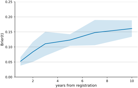
Lower is better. The Brier score combines discrimination (does the model rank patients correctly) and calibration (are the absolute probabilities right) into one number per horizon; integrated over a window it becomes the Integrated Brier Score (IBS), available as ts.metrics.brier.integrated. The mean Brier score rises from 0.05 at one year to 0.16 at ten, and the band shows one standard deviation across the five folds.
Limitations
Section titled “Limitations”- Proportional hazards: The Cox model assumes the hazard ratio for each covariate is constant over time. PBC may violate this for bilirubin and stage at long follow-up; a check based on Schoenfeld residuals is not covered here.
- Competing risks: Liver transplant was treated as censoring in the single-event recoding. That is the standard simplification, but it conflates “we stopped watching” with “the patient received a transplant, which changes their prognosis.” The competing-risks tutorial revisits this using
ts.linear.FineGrayand the cause-specific cumulative incidence. - Evaluation: The 70/30 split here is the simplest possible. A reporting pipeline uses repeated cross-validation, bootstraps the calibration curves, and reports the integrated Brier score and time-dependent AUC alongside the Brier score. Cross-validate and tune a model covers the cross-validation part.
- Causal interpretation: A hazard ratio is a population summary, not a causal effect of changing a covariate. The separate
causurvpackage covers what additional assumptions are needed before HRs become causal contrasts and why RMST differences are often a cleaner target.
References
Section titled “References”- Therneau, T. & Grambsch, P. (2000). Modeling Survival Data: Extending the Cox Model. Springer.
- Cox, D. R. (1972). Regression models and life-tables. Journal of the Royal Statistical Society, Series B 34(2).
- Breslow, N. (1974). Covariance analysis of censored survival data. Biometrics 30(1).
- Graf, E., Schmoor, C., Sauerbrei, W. & Schumacher, M. (1999). Assessment and comparison of prognostic classification schemes for survival data. Statistics in Medicine 18.
- Krzyziński, M., Spytek, M., Baniecki, H. & Biecek, P. (2023). SurvSHAP(t): time-dependent explanations of machine learning survival models. Knowledge-Based Systems 262, 110234.