Competing risks
Set up
Section titled “Set up”import matplotlib.pyplot as pltimport numpy as npimport polars as pl
import tausurv as ts
%config InlineBackend.figure_format = 'svg'
ts.plot.set_style("publication")Bringing the competing event back
Section titled “Bringing the competing event back”ts.datasets.load_pbc() returns the single-event bunch. The pbc:transplant variant reads the same 418 patients as competing risks, coded with the convention used throughout the library: cause 0 is censored, cause 1 is the event of interest (death), cause 2 is the competing event (transplant).
pbc = ts.datasets.load_dataset("pbc:transplant")X_full, Y_full, _ = pbcY_full = Y_full / 365.25  # days -> yearsevent = pbc.cause
counts = pl.DataFrame(    {        "outcome": ["censored", "death", "transplant"],        "n": [            int((event == 0).sum()),            int((event == 1).sum()),            int((event == 2).sum()),        ],    })counts
shape: (3, 2) ┌────────────┬─────┐ │ outcome ┆ n │ │ --- ┆ --- │ │ str ┆ i64 │ ╞════════════╪═════╡ │ censored ┆ 232 │ │ death ┆ 161 │ │ transplant ┆ 25 │ └────────────┴─────┘
25 of the 418 patients (6%) received a transplant. The single-event recoding counted them as censored, although their outcome is known.
The pitfall: overstates the cause incidence
Section titled “The pitfall: 1−KM^1 - \widehat{\mathrm{KM}}1−KM overstates the cause incidence”Computing Kaplan-Meier with death as the event and transplant as censoring, then reporting as the incidence of death, overestimates that incidence whenever the competing event occurs. Censoring assumes the transplanted patients could still die later at the rate of those still at risk, so their future deaths are counted although they never happen as first events.
The Aalen-Johansen estimator estimates the probability of an event of cause by time with the competing cause present.
death_or_not = (event == 1).astype(np.int8)S_naive = ts.nonparametric.kaplan_meier(Y_full, death_or_not)F_aj = ts.nonparametric.aalen_johansen(Y_full, event, cause=1)
t_grid = np.linspace(0.1, 12.0, 240)naive_cif = 1.0 - S_naive(t_grid)aj_cif = F_aj(t_grid)
fig, ax = plt.subplots()ax.step(    t_grid,    naive_cif,    where="post",    label=r"$1 - \widehat{\mathrm{KM}}$ (transplant as censoring)",)ax.step(t_grid, aj_cif, where="post", label="Aalen-Johansen $\\hat F_\\mathrm{death}$")ax.set_xlabel("years from registration")ax.set_ylabel("cumulative incidence of death")ax.set_xlim(0, 12)ax.set_ylim(0, None)ax.legend(loc="lower right")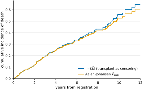
The one-minus-Kaplan-Meier curve never falls below the Aalen-Johansen curve, and the gap grows with time: 0.297 against 0.292 at five years, 0.558 against 0.527 at ten. The gap is small here because only 6% of patients had a transplant; it grows with the rate of the competing event (Andersen et al. 2012).
Both causes at once
Section titled “Both causes at once”ts.plot.cif draws one Aalen-Johansen curve per cause, with an at-risk table aligned to the time axis as in ts.plot.km.
ts.plot.cif( Y_full, event, cause_labels={1: "death", 2: "transplant"}, xlabel="years from registration",)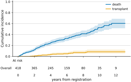
By ten years the cumulative incidence is 0.53 for death and 0.08 for transplant; one minus their sum is the probability of being alive without a transplant.
Fitting a Fine-Gray model for death
Section titled “Fitting a Fine-Gray model for death”The Fine-Gray model parameterises the subdistribution hazard of a chosen cause:
Subjects with a competing event stay in the risk set, with a weight that decreases with the estimated probability of remaining uncensored; in a cause-specific Cox model they would leave it. A positive coefficient therefore raises the cumulative incidence curve of the cause, and a negative one lowers it. The covariates and the train/test split are those of the previous tutorial.
keep = ["age", "sex", "stage", "bili", "albumin"]df = X_full.select(keep).with_row_index("_row").drop_nulls()kept = df["_row"].to_numpy()df = (    df.drop("_row")    .with_columns(sex_male=(pl.col("sex") == "m").cast(pl.Int8))    .drop("sex")    .select(["age", "stage", "bili", "albumin", "sex_male"]))X_array = df.to_numpy().astype(np.float64)event_kept = event[kept]Y_kept = Y_full[kept]feature_names = list(df.columns)
rng = np.random.default_rng(seed=42)order = rng.permutation(len(Y_kept))split = int(0.7 * len(Y_kept))train, test = order[:split], order[split:]
fg = ts.linear.FineGray(cause=1).fit(X_array[train], Y_kept[train], event_kept[train])
print(    f"train: n = {len(train)}, deaths = {int((event_kept[train] == 1).sum())}, "    f"transplants = {int((event_kept[train] == 2).sum())}")
train: n = 288, deaths = 109, transplants = 17
A subdistribution hazard ratio (SHR) multiplies the subdistribution hazard, not the cause-specific hazard. An SHR of 1.5 for stage means that a higher stage raises the cumulative incidence of death; it does not mean that the death rate among patients still alive and untransplanted is 1.5 times higher.
ts.plot.forest( names=feature_names, estimates=np.exp(fg.coef_), xlabel="Subdistribution hazard ratio (Fine-Gray)",)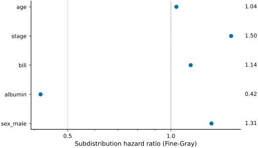
The SHRs are 1.50 per stage, 1.14 per mg/dL of bilirubin, 1.04 per year of age, 1.31 for male sex and 0.42 per g/dL of albumin, close to the Cox hazard ratios of the previous tutorial because transplants are rare in this cohort. The two ratios answer different questions and are often confused: of 55 papers reporting Fine-Gray models, Austin & Fine (2017) found 5 that interpreted the SHRs correctly.
Predicting cumulative incidence for two patients
Section titled “Predicting cumulative incidence for two patients”predict_cif returns at the requested times, here for the early-stage and the advanced profile of the Cox tutorial.
profiles = {    "Early PBC, age 50, normal labs": np.array([50.0, 1.0, 0.6, 4.0, 0.0]),    "Advanced PBC, age 70, abnormal labs": np.array([70.0, 4.0, 8.0, 2.8, 0.0]),}times_pred = np.linspace(0.1, 12.0, 240)F_pred = fg.predict_cif(np.stack(list(profiles.values())), times_pred)
fig, ax = plt.subplots()for label, f in zip(profiles, F_pred, strict=True):    ax.step(times_pred, f, where="post", label=label)ax.set_xlabel("years from registration")ax.set_ylabel(r"$\hat F_\mathrm{death}(t \mid x)$")ax.set_xlim(0, 12)ax.set_ylim(0, 1.0)ax.legend(loc="lower right")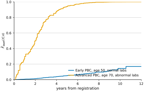
The predicted cumulative incidence of death is 0.94 at five years for the advanced profile and 0.05 for the early one; at ten years it is 1.00 and 0.14. These numbers answer “what proportion of patients like this die by year ” directly.
How well does the model fit?
Section titled “How well does the model fit?”ts.metrics.brier.score_cause_specific scores predicted cumulative incidences against the observed events of one cause; it is the competing-risks counterpart of the Brier score in the Cox tutorial.
horizons = np.array([1.0, 2.0, 3.0, 5.0, 7.0, 10.0])F_test = fg.predict_cif(X_array[test], horizons)
brier_cs = ts.metrics.brier.score_cause_specific(    Y_kept[test], event_kept[test], F_test, horizons, cause=1)
ts.plot.brier_over_time(    horizons,    brier_cs,    xlabel="years from registration",    ylabel="Brier score (cause-specific, death)",)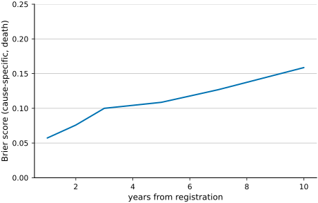
Lower is better. The score rises from 0.06 at one year to 0.16 at ten, on the 124 test patients.
Limitations
Section titled “Limitations”- Reporting: an SHR is not a cause-specific hazard ratio. Austin & Fine (2017) give recommendations for reporting Fine-Gray analyses; state which ratio a result is.
- Cause-specific hazards: for the question “which covariates raise the death rate among patients still at risk”, a Cox model with transplant as censoring estimates the cause-specific hazard. Latouche et al. (2013) recommend reporting the cause-specific hazards and the cumulative incidence functions of all causes.
- Several causes: Fine-Gray models fitted separately for each cause can predict cumulative incidences that sum to more than 1 (Austin, Putter, Lee & Steyerberg 2022). To predict the incidence of every cause, use cause-specific hazard models.
- Causal interpretation: the covariates are not randomised, and the SHRs describe associations, not causal effects. The separate
causurvpackage covers the assumptions under which survival contrasts have a causal meaning.
References
Section titled “References”- Fine, J. P. & Gray, R. J. (1999). A proportional hazards model for the subdistribution of a competing risk. Journal of the American Statistical Association 94(446), 496-509.
- Andersen, P. K., Geskus, R. B., de Witte, T. & Putter, H. (2012). Competing risks in epidemiology: possibilities and pitfalls. International Journal of Epidemiology 41(3), 861-870.
- Latouche, A., Allignol, A., Beyersmann, J., Labopin, M. & Fine, J. P. (2013). A competing risks analysis should report results on all cause-specific hazards and cumulative incidence functions. Journal of Clinical Epidemiology 66(6), 648-653.
- Austin, P. C. & Fine, J. P. (2017). Practical recommendations for reporting Fine-Gray model analyses for competing risk data. Statistics in Medicine 36(27), 4391-4400.
- Austin, P. C., Putter, H., Lee, D. S. & Steyerberg, E. W. (2022). Estimation of the absolute risk of cardiovascular disease and other events: issues with the use of multiple Fine-Gray subdistribution hazard models. Circulation: Cardiovascular Quality and Outcomes 15(2), e008368.