Styling

import numpy as np
import matplotlib.pyplot as plt

import tausurv as ts

%config InlineBackend.figure_format = 'svg'

rng = np.random.default_rng(0)
t = np.linspace(0.1, 5.0, 100)
S = {
    "control": np.exp(-0.35 * t),
    "treatment": np.exp(-0.18 * t),
}

The four named styles

Each preset is a set of rcParams. All presets use the same palette (Okabe-Ito by default), so colours match across contexts.

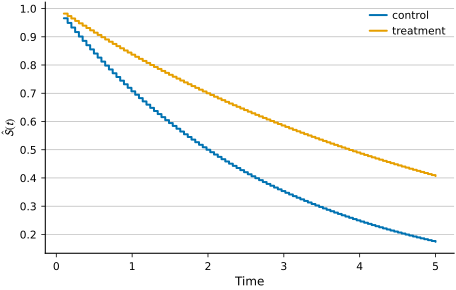
publication

The default. Single-column journal width (~5.5 in), 9 pt body font, restrained spines (no top / no right), light y-only gridlines, line width 1.5.

ts.plot.set_style("publication")
fig, ax = plt.subplots()
for name, curve in S.items():
    ax.step(t, curve, where="post", label=name)
ax.set_xlabel("Time")
ax.set_ylabel(r"$\hat S(t)$")
ax.legend()
fig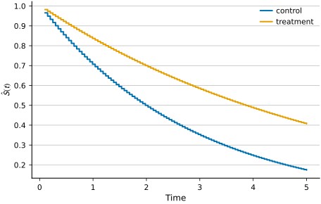

presentation

Slides and posters. 13 pt body font, 2.5 pt lines, larger figure (8 × 5 in), 120 DPI.

ts.plot.set_style("presentation")
fig, ax = plt.subplots()
for name, curve in S.items():
    ax.step(t, curve, where="post", label=name)
ax.set_xlabel("Time")
ax.set_ylabel(r"$\hat S(t)$")
ax.legend()
fig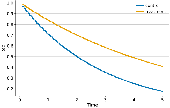

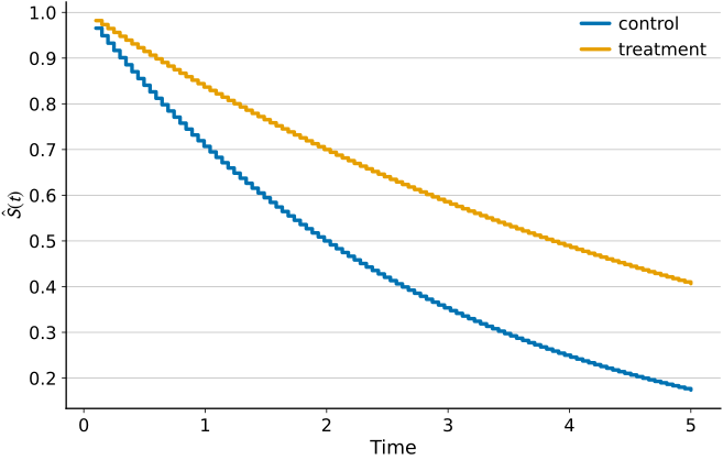
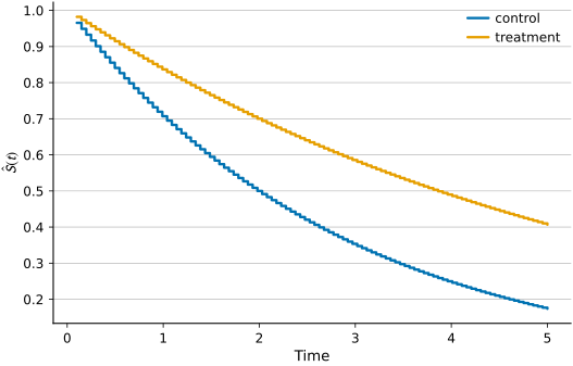
notebook

Interactive analysis. Matplotlib’s default proportions (6.4 × 4 in) with the tausurv palette and minor spine / grid cleanup.

ts.plot.set_style("notebook")
fig, ax = plt.subplots()
for name, curve in S.items():
    ax.step(t, curve, where="post", label=name)
ax.set_xlabel("Time")
ax.set_ylabel(r"$\hat S(t)$")
ax.legend()
fig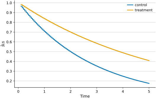

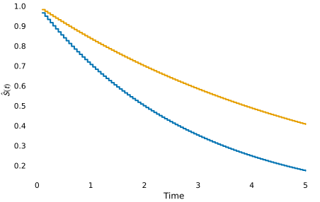
minimal

No spines, no gridlines, lines only. For embedding figures in mixed-media reports where the surrounding context provides axes, or for sparkline-style overviews.

ts.plot.set_style("minimal")
fig, ax = plt.subplots()
for name, curve in S.items():
    ax.step(t, curve, where="post", label=name)
ax.set_xlabel("Time")
ax.set_ylabel(r"$\hat S(t)$")
fig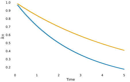

Restore the default for the rest of the page.

ts.plot.set_style("publication")

Palettes

The module has three categorical palettes. The default is Okabe-Ito (Okabe & Ito 2008): eight colours, distinguishable under colour-vision deficiency. Several pairs have the same lightness, so in grayscale print add line styles or markers.

def palette_swatch(name, colours):
    fig, ax = plt.subplots(figsize=(5.5, 0.6))
    ax.set_axis_off()
    n = len(colours)
    for i, c in enumerate(colours):
        ax.add_patch(plt.Rectangle((i, 0), 1, 1, facecolor=c, edgecolor="none"))
    ax.set_xlim(0, n)
    ax.set_ylim(0, 1)
    ax.set_title(name, loc="left", fontsize=10, pad=4)
    fig.tight_layout()
    return fig


palette_swatch("Okabe-Ito (default)", ts.plot.colors.OKABE_ITO)

Two alternates are available for slides, posters, or competing-risks stacks where you want a palette distinct from Okabe-Ito to avoid colour clashes:

palette_swatch("Tol Bright", ts.plot.colors.TOL_BRIGHT)

palette_swatch("Tol Muted", ts.plot.colors.TOL_MUTED)

For two-group treatment-vs-control plots the natural pair is the first two Okabe-Ito colours — blue and orange — which are accessed via a dedicated helper:

control, treatment = ts.plot.colors.treatment_control()
print(f"control:   {control}")
print(f"treatment: {treatment}")

control:   #0072B2
treatment: #E69F00

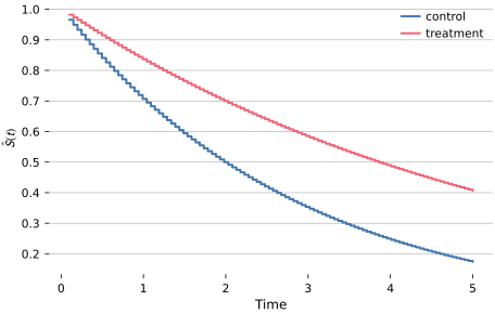
Switch the active palette via the palette= argument to set_style:

ts.plot.set_style("publication", palette="tol_bright")
fig, ax = plt.subplots()
for name, curve in S.items():
    ax.step(t, curve, where="post", label=name)
ax.set_xlabel("Time")
ax.set_ylabel(r"$\hat S(t)$")
ax.legend()
fig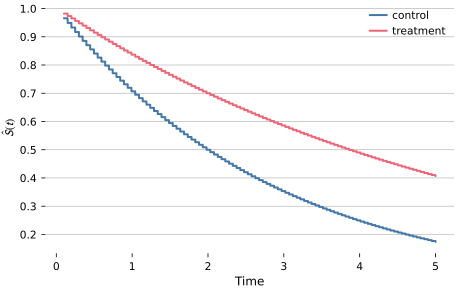

ts.plot.set_style("publication")  # restore default

Scoped style with style_context

When you only need a style for one figure — a presentation-sized export from an otherwise publication-styled notebook, say — use the context manager instead of mutating set_style globally.

with ts.plot.style_context("presentation"):
    fig, ax = plt.subplots()
    for name, curve in S.items():
        ax.step(t, curve, where="post", label=name)
    ax.set_xlabel("Time")
    ax.set_ylabel(r"$\hat S(t)$")
    ax.legend()
fig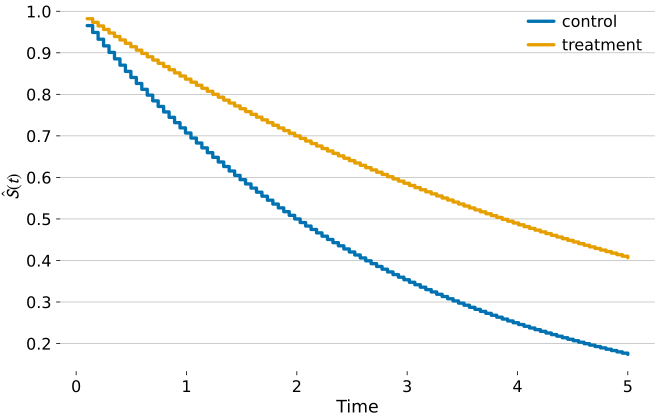

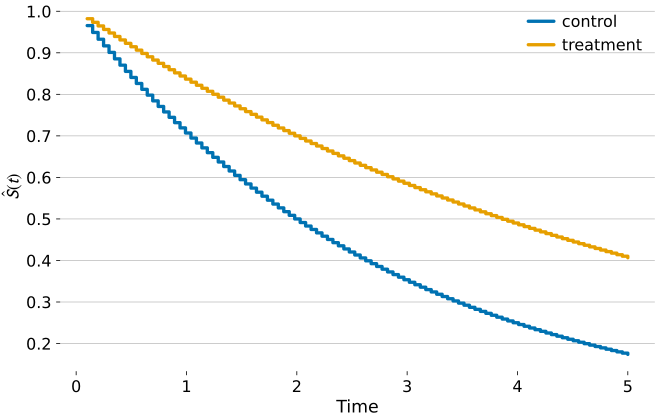
After the with block, the previous style is restored.

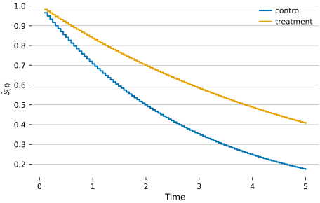
fig, ax = plt.subplots()
for name, curve in S.items():
    ax.step(t, curve, where="post", label=name)
ax.set_xlabel("Time")
ax.set_ylabel(r"$\hat S(t)$")
ax.legend()
fig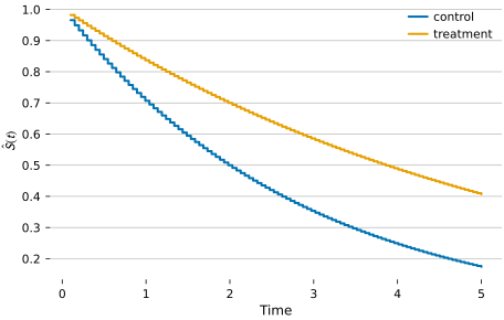

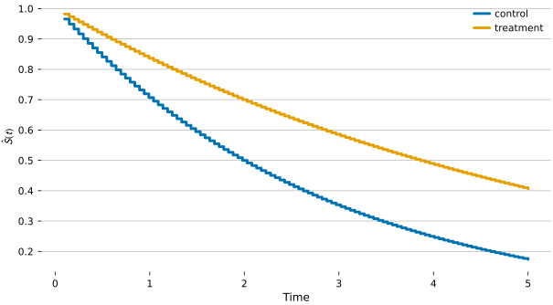
Per-call overrides

Both set_style and style_context accept arbitrary rcParams as keyword arguments, applied last. Use them for one-off tweaks (a wider figure, a heavier line) without writing a new named style.

with ts.plot.style_context(
    "publication",
    **{"figure.figsize": (7.5, 4.0), "lines.linewidth": 2.2},
):
    fig, ax = plt.subplots()
    for name, curve in S.items():
        ax.step(t, curve, where="post", label=name)
    ax.set_xlabel("Time")
    ax.set_ylabel(r"$\hat S(t)$")
    ax.legend()
fig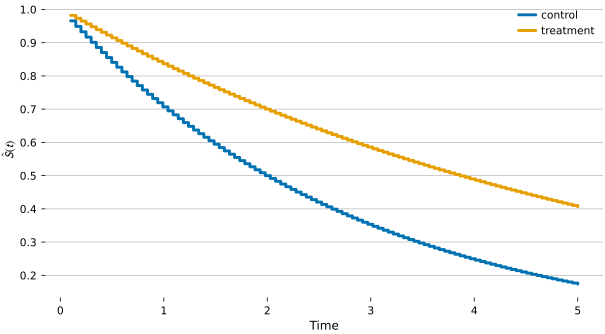

Font fallbacks

The publication and presentation styles ship a wide fallback chain: Source Sans 3 → IBM Plex Sans → Inter → Roboto → Open Sans → Helvetica → Arial → DejaVu Sans. Whichever the system has, matplotlib will land on it. The figures on this page render with whatever font is available on the docs build host; on Linux without optional fonts installed that’s typically DejaVu Sans, which is bundled with matplotlib.