Quickstart

The code below fits and plots a Kaplan-Meier survival curve on the Mayo Clinic primary biliary cholangitis (PBC) trial cohort, with a logit-transformed 95% confidence band and an at-risk table aligned to the time axis.

import tausurv as ts

ts.plot.set_style("publication")
X, Y, delta = ts.datasets.load_pbc()
ts.plot.km(Y / 365.25, delta, xlabel="years from registration")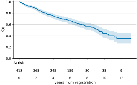

ts.datasets.load_pbc() returns a SurvivalBunch that tuple-unpacks as (X, Y, delta): a polars DataFrame of covariates, the observed time $Y = \min(T, C)$ in days, and the event indicator $\delta$. The dataset downloads on first call and caches locally; subsequent runs read from the user cache directory (~/.cache/tausurv/datasets/ on Linux). ts.plot.set_style("publication") configures matplotlib once for the rest of the session: sans-serif font, single accent colour, no top or right spines, Okabe-Ito palette.

What you need

• Python ≥ 3.12
• pip install tausurv[plot] for matplotlib-backed plotting (the plot extra is optional but everything in this Quickstart needs it)
• Internet on first run for the dataset download (set TAUSURV_OFFLINE=1 to make the fetch raise instead)

Where next

• Tutorial 1: Your first survival analysis takes the analysis above further: median survival, treatment-arm comparison, stratification by histologic stage.
• Tutorial 2: Modeling risk with covariates fits a Cox model on the same cohort, with hazard-ratio interpretation, SHAP decomposition for an individual prediction, and held-out calibration and Brier evaluation.
• Tutorial 3: Competing risks brings the third outcome back (transplant), shows why applying $1 - \widehat{\mathrm{KM}}$ to one cause overstates incidence, and fits a Fine-Gray model.
• Thinking in survival explains censoring, the at-risk set and the choice of quantity to estimate, before any method.