Thinking in survival

Survival analysis is the set of methods for data where the event of interest does not happen for every subject you observe. Two choices come before any method: which quantity to estimate, and which assumption the estimate rests on.

The data

You have records of people, customers, machines, or any other unit observed over time. For each one you know either when an event happened (a death, a churn, a failure) or only that nothing had happened by the time you stopped watching. The second case is called censoring.

Take six patients followed for up to five years. Their records look like this:

subject	$y_i$ (years)	$\delta_i$
A	1.0	1
B	1.8	0
C	3.0	1
D	4.0	0
E	4.5	1
F	5.0	0

$y_i$ is the observed time, the smaller of the event time and the last contact time. $\delta_i$ is one if the event was observed, zero otherwise. The pair $(Y, \delta)$ is the input every method in tausurv expects.

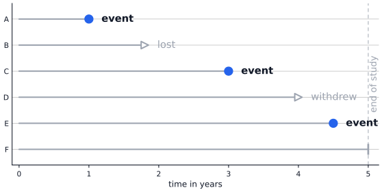
Source

"""Six patients followed for up to five years, each ending in a different fate.

Used in the "Thinking in Survival" concept page to introduce the (Y, delta)
data layout, the at-risk set, and the visual taxonomy of censoring.
"""

from __future__ import annotations

from pathlib import Path

import matplotlib.pyplot as plt
from _style import ACCENT, INK, MUTED, setup_style


def make(out_path: Path) -> None:
    setup_style()

    subjects = [
        ("A", 1.0, "event"),
        ("B", 1.8, "lost"),
        ("C", 3.0, "event"),
        ("D", 4.0, "withdrew"),
        ("E", 4.5, "event"),
        ("F", 5.0, "admin"),
    ]
    n = len(subjects)
    end_of_study = 5.0

    fig, ax = plt.subplots(figsize=(7.2, 3.2))

    ax.axvline(
        end_of_study,
        color=MUTED,
        linestyle=(0, (4, 3)),
        linewidth=1.0,
        alpha=0.7,
        zorder=1,
    )
    ax.text(
        end_of_study + 0.08,
        (n + 1) / 2,
        "end of study",
        color=MUTED,
        rotation=90,
        ha="center",
        va="center",
        fontsize=10,
    )

    for idx, (_label, y_i, kind) in enumerate(subjects):
        row = idx + 1
        ax.plot([0, y_i], [row, row], color=MUTED, linewidth=1.5, zorder=2)
        if kind == "event":
            ax.plot(
                y_i,
                row,
                "o",
                markerfacecolor=ACCENT,
                markeredgecolor=ACCENT,
                markersize=9,
                zorder=3,
            )
            ax.text(
                y_i + 0.18,
                row,
                "event",
                color=INK,
                fontweight="bold",
                va="center",
                fontsize=11,
            )
        elif kind == "admin":
            ax.plot(
                y_i,
                row,
                "|",
                color=MUTED,
                markersize=12,
                markeredgewidth=2.0,
                zorder=3,
            )
        else:
            ax.plot(
                y_i,
                row,
                ">",
                markerfacecolor="white",
                markeredgecolor=MUTED,
                markersize=8,
                markeredgewidth=1.5,
                zorder=3,
            )
            ax.text(
                y_i + 0.18,
                row,
                kind,
                color=MUTED,
                va="center",
                fontsize=11,
            )

    ax.set_yticks(range(1, n + 1))
    ax.set_yticklabels([s[0] for s in subjects])
    ax.set_xticks([0, 1, 2, 3, 4, 5])
    ax.set_xlim(-0.1, 5.15)
    ax.set_ylim(0.4, n + 0.6)
    ax.invert_yaxis()
    ax.set_xlabel("time in years")
    ax.tick_params(axis="y", length=0)

    fig.savefig(out_path, bbox_inches="tight", pad_inches=0.05)
    plt.close(fig)


if __name__ == "__main__":
    out = (
        Path(__file__).resolve().parent.parent
        / "public"
        / "figures"
        / "thinking_swimmer.svg"
    )
    out.parent.mkdir(parents=True, exist_ok=True)
    make(out)

Why naive arithmetic fails

A spreadsheet might be tempted to take the mean of $y_i$ and call it average survival. That mean is about 3.22 years. It is wrong as a survival summary, because three of the six patients (B, D, F) are censored: their true event times are at least the recorded ones, and may be substantially greater. The naive average is a lower bound on the truth, not the truth.

A more careful question is the probability of being event-free at three years. Three patients have $y_i > 3$ (D, E, F), so a naive answer is $3/6 = 0.5$. But patient B was lost to follow-up at $y_B = 1.8$. We do not know whether B was event-free at year three; we only know B was event-free at year 1.8. Counting B as a non-survivor (which is what the naive $0.5$ does) is a guess, not a measurement.

A correct answer needs a rule for how censored subjects count, and an assumption about what happens to them after censoring.

The at-risk set

The fundamental object is the at-risk set. At any time $t$, the at-risk set is the set of subjects who have been observed up to just before $t$ and have not yet had the event.

For the six patients above:

• At $t = 0$: all six are at risk.
• At $t = 1.0$: patient A has the event. The at-risk set shrinks to five.
• At $t = 1.8$: patient B is lost to follow-up. The at-risk set shrinks to four, but not because of an event.
• At $t = 3.0$: patient C has the event. The at-risk set shrinks to three.
• At $t = 4.0$: patient D withdraws. The at-risk set shrinks to two.
• At $t = 4.5$: patient E has the event. The at-risk set shrinks to one.
• At $t = 5.0$: patient F reaches the end of the study without an event.

Every nonparametric estimator in tausurv is a function of how the at-risk set evolves. Kaplan-Meier multiplies survival across the times when events occurred. Nelson-Aalen accumulates the ratio of events to at-risk count. Aalen-Johansen does the same with multiple causes. The bookkeeping is the same; the estimand differs.

The Kaplan-Meier estimate of the survival function is the running product

$$\hat S(t) = \prod_{t_k \le t} \left(1 - \frac{d_k}{n_k}\right),$$

where $t_k$ are the times at which events occurred, $d_k$ is the number of events at $t_k$, and $n_k$ is the at-risk count just before $t_k$. Just after patient C’s event:

$$\hat S(3) \;=\; \frac{5}{6} \cdot \frac{3}{4} \;=\; \frac{5}{8} \;=\; 0.625.$$

The naive $0.5$ was wrong because it treated patient B as a failure for being lost to follow-up. The Kaplan-Meier $0.625$ keeps B in the at-risk set up to $1.8$ and then drops B without counting against survival.

Same data, different questions

The number we just computed, $\hat S(3) = 0.625$, is the probability of being event-free at three years. The same table answers other questions, and each lands on its own object.

What fraction is event-free at five years? is a probability question, answered by the survival function $S(t)$. What is the rate of failure? is a rate question, answered by the hazard $\lambda(t)$. What is the expected event-free time over the next two years? is a time question, answered by the restricted mean survival time $\mu(\tau)$. A fourth object, the cumulative hazard $\Lambda(t)$, is used inside many methods and for diagnostics.

Survival probability $S(t)$

The survival function $S(t) = P(T > t)$ is the probability that a subject has not had the event by time $t$. It starts at one and falls toward zero.

Reach for $S(t)$ when the audience will read the result as an absolute probability at a chosen time:

• A clinical-trial paper reports “five-year recurrence-free survival was 78%”. That number is $\hat S(5\text{ years})$ for the trial cohort.
• A retention team reports “65% of customers are still subscribed twelve months after sign-up”. That is $\hat S(12\text{ months})$ on a churn cohort.
• An actuary publishes “life-table survival from age 65”: $\hat S$ on an age time-scale.

In our six-patient example, $\hat S(3) = 0.625$. The estimated probability that a subject is event-free three years after enrollment is about 63%.

Hazard rate $\lambda(t)$

The hazard rate $\lambda(t)$ is the instantaneous rate of failure at $t$, given survival to $t$. Its units are per-time, not probability. A hazard of $0.1$ per year does not mean “10% chance of failure”. It means that in any short window $[t, t + dt]$, the conditional probability of failure is approximately $\lambda(t)\,dt$.

Reach for $\lambda(t)$ when:

• You want to compare risk between groups in a regression model. The Cox model parameterises how covariates multiply $\lambda$; a hazard ratio of $1.5$ means “the instantaneous rate is 1.5 times higher in this group”.
• “Rate per unit time” is the conventional language of your domain: events per 1000 person-years in epidemiology, failures per operating hour in reliability, defaults per year in credit risk.
• You want to see when risk is changing. An early-rising hazard suggests an acute effect; a declining hazard suggests the high-risk subjects are weeded out early; a bathtub shape is the reliability-engineering signature of infant mortality plus wear-out.

Common trap: reading $\lambda(t)$ as a probability. It can be greater than one.

Cumulative hazard $\Lambda(t)$

The cumulative hazard is the integrated hazard: $\Lambda(t) = \int_0^t \lambda(u)\,du$. Roughly, it is the total risk accumulated by time $t$. The identity $S(t) = e^{-\Lambda(t)}$ ties it back to $S$.

For single-event survival, most readers meet $\Lambda$ indirectly. It is the working object inside Cox regression and the natural target of Nelson-Aalen, but it is rarely the decision-facing quantity that $S$, $\lambda$, or $\mu(\tau)$ are. The cases where you reach for $\Lambda$ directly are narrower but real:

• You are tracking recurrent events, not first-event time. For hospital readmissions, machine breakdowns with repair, repeat insurance claims, or customer complaints, the decision-facing quantity is the expected cumulative count of events by time $t$. Nelson-Aalen estimates this directly. A hospital quality team reads $\hat\Lambda(\text{30 days}) = 0.43$ as “an average of 0.43 readmissions per discharged patient within 30 days”, a number a hospital administrator acts on.
• You are choosing a parametric failure distribution to fit. Plotting $\hat\Lambda(t)$ on linear axes shows whether the hazard is constant (a straight line through the origin says exponential); plotting it on log-log axes shows whether the data are Weibull (a straight line). Reliability engineers use this visual diagnostic to choose between Weibull, log-normal, and exponential models before committing to one.
• You are working with a multi-state or additive-hazard framework. Disease progression (well → disabled → dead), customer state machines (trial → active → at-risk → churned), credit-cycle transitions: each transition has its own cumulative intensity $\Lambda_{jk}(t)$. Aalen’s additive-hazard model adds covariate effects directly to $\Lambda$, which keeps time-varying effects easier to interpret than on the multiplicative $\lambda$ scale.

Restricted mean survival time $\mu(\tau)$

The restricted mean survival time is the average event-free time within a horizon $\tau$:

$$\mu(\tau) = \int_0^\tau S(t)\,dt.$$

In words: of the next $\tau$ years, how many does a typical subject spend event-free? RMST has the same units as time and always exists for any $\tau$ within follow-up.

Reach for RMST when:

• You want a single interpretable summary in time units. “Treatment-arm patients have an average of 14.2 event-free months over the next 24 months, compared to 12.1 in the control arm” is an RMST contrast.
• The median survival time is not estimable because more than half the cohort is still event-free at the end of follow-up. RMST does not need the curve to drop below 0.5.
• The treatment effect has a time course. Immunotherapies that take six months to start working; drugs that change the long-term curve but not the short-term hazard; infrastructure investments that pay off after a multi-year delay. The hazard ratio assumes the effect is a constant multiplier of the rate at every time. When that’s not true, the RMST contrast captures the cumulative time gained over the horizon and the HR averages the shape away.
• You need to feed survival into a downstream economic computation. Quality-adjusted life years (QALY) in health economics, customer lifetime value (LTV) in retention, expected service hours in reliability: all of these integrate against $S$ on a horizon, which is RMST.

Choice of $\tau$ matters. $\mu(2)$ and $\mu(5)$ are different numbers. Compare RMSTs at the same $\tau$.

Decision table

Decision	Quantity	Concrete example
Communicate absolute risk at a horizon	$S(t)$	”73% alive at five years”
Compare groups by regression	$\lambda(t)$	Cox hazard ratio of 1.5 between treatment arms
Summarise in time units, or contrast under non-PH	$\mu(\tau)$	”14 of 24 months event-free, treatment vs 12 control”
Diagnose model fit, or do additive decomposition	$\Lambda(t)$	$\hat\Lambda$ linear on log-log axes implies Weibull

Competing events change the question

A second event type can make the event of interest impossible. In an older patient cohort, death from any cause makes future cancer relapse unobservable. In credit risk, loan prepayment ends the window in which default could occur. In transplantation, non-relapse mortality ends the window in which relapse could occur.

These are not censoring. The competing event happened. The subject is not still at risk.

Treating a competing event as censoring and running Kaplan-Meier overstates the incidence, and the bias grows with the rate of the competing event. The correct nonparametric object is the cumulative incidence function

$$F_j(t) = P(T \le t,\; J = j),$$

the probability of failing from cause $j$ by time $t$. It is estimated by Aalen-Johansen. Andersen et al. (2012) show the bias of $1 - \text{KM}$ per cause on a transplant cohort.

The assumption every estimate carries

Each method above relies on at least one condition that the data cannot verify. For nonparametric survival estimation, the central condition is independent censoring: the censoring time is independent of the event time, possibly after conditioning on covariates.

When subjects who are at higher risk drop out of follow-up for reasons related to that risk, the condition fails. Every estimate produced from the data is biased, and the bias is not detectable from $(Y, \delta)$ alone. Tsiatis showed in 1975 that the joint distribution of event and censoring times is not identifiable from the observed data, even in principle.

Whether the assumption is plausible depends on why subjects are censored.

1. If the reason a subject is censored is unrelated to their underlying state (administrative end of follow-up, the study closing, a customer’s contract ending on a fixed date), the assumption is plausible.
2. If the reason is plausibly related (loss to follow-up because the patient got sicker and stopped attending, a customer churning quietly without being recorded), the assumption is suspect. Run diagnostics, consider methods that condition on richer covariates, and report a sensitivity envelope.

Report the assumption together with the estimate it supports.

How to use this mental model

Four questions to answer before choosing a method:

1. What is the decision? A clinician choosing a treatment needs absolute risk at a fixed horizon. An epidemiologist comparing populations needs an effect estimate. A health economist building a model needs an integral over time. A retention team needs a cohort curve. Different decisions, different quantities.
2. What is the estimand? Survival at $t$, cumulative incidence of cause $j$, restricted mean survival, hazard ratio, counterfactual survival under treatment. Name it before you pick a method.
3. What can the data identify? Marginal $S(t)$ under independent censoring. Cumulative incidence under independent administrative censoring. Cause-specific hazards. The hazard ratio as a population summary, not a causal contrast. Some quantities (net survival, the latent marginal distribution of $T$ in the presence of dependent censoring) cannot be identified from $(Y, \delta)$ data alone.
4. What assumption am I willing to make, and how would I know if it broke? Independent censoring is the smallest assumption. Conditional independent censoring given covariates is the next step. Parametric copula, joint longitudinal-event modeling, sensitivity bounds are the steps beyond.

Where to go from here

The tutorials apply these ideas to the PBC trial: Kaplan-Meier curves, a Cox model, and competing risks with Aalen-Johansen and Fine-Gray.

References

• Aalen O, Borgan Ø, Gjessing H (2008). Survival and Event History Analysis. Springer. The modern counting-process treatment.
• Andersen PK, Geskus RB, de Witte T, Putter H (2012). Competing risks in epidemiology: possibilities and pitfalls. International Journal of Epidemiology 41:861–870. Shows the bias of Kaplan-Meier applied to one of several competing causes.
• Kaplan EL, Meier P (1958). Nonparametric estimation from incomplete observations. JASA 53:457–481. The Kaplan-Meier paper.
• Klein JP, Moeschberger ML (2003). Survival Analysis: Techniques for Censored and Truncated Data. Springer. The applied standard reference.
• Tsiatis A (1975). A nonidentifiability aspect of the problem of competing risks. PNAS 72:20–22. The non-identifiability result cited in the section on assumptions.