Your first survival analysis

Set up

Throughout the docs we import tausurv as ts and access subpackages explicitly (ts.datasets, ts.nonparametric, ts.plot). The convention mirrors numpy as np and pandas as pd and keeps the library structure visible at the call site. ts.plot.set_style("publication") sets the matplotlib style once for the session.

import numpy as np

import tausurv as ts

%config InlineBackend.figure_format = 'svg'

ts.plot.set_style("publication")

The PBC trial cohort

The Mayo Clinic primary biliary cholangitis trial (1974-1984) followed 418 patients with PBC liver disease. The first 312 were randomised to D-penicillamine or placebo; the remaining 106 are non-randomised follow-up. The outcome is time to death, in days. Following the standard single-event recoding, liver transplants and end-of-study are treated as censoring.

ts.datasets.load_pbc() returns a SurvivalBunch that tuple-unpacks as (X, Y, delta). The bunch also carries metadata (.name, .description, .citation).

pbc = ts.datasets.load_pbc()
X, Y, delta = pbc

# Convert days to years for a more readable time axis.
Y = Y / 365.25

n = len(Y)
n_events = int(delta.sum())
print(f"{n} patients, {n_events} deaths ({n_events / n:.0%})")
print(f"median follow-up: {np.median(Y):.2f} years")
print(f"covariates ({X.width}): {', '.join(X.columns)}")

418 patients, 161 deaths (39%)
median follow-up: 4.74 years
covariates (17): trt, age, sex, ascites, hepato, spiders, edema, bili, chol, albumin, copper, alk.phos, ast, trig, platelet, protime, stage

Beyond (Y, delta), PBC carries the treatment arm (trt, 1 = D-penicillamine, 2 = placebo, null = non-randomised follow-up), demographics (age, sex), lab values measured at trial entry (bili for bilirubin, albumin, chol, copper, …), and the histologic disease stage (stage, 1-4, higher is worse). This tutorial uses trt and stage.

Overall survival

ts.plot.km on raw $(Y, \delta)$ arrays fits Kaplan-Meier internally and draws by default a pointwise 95% confidence band computed on the logit scale, which keeps it inside $[0, 1]$, and an at-risk table aligned to the time axis (Pocock, Clayton & Altman, Lancet 2002).

ts.plot.km(Y, delta, xlabel="years from registration")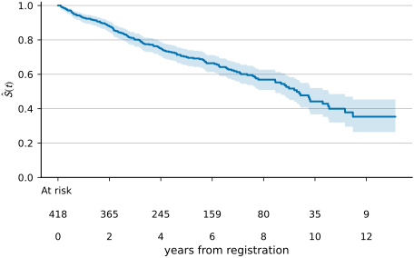

The Kaplan-Meier estimate is a StepFunction: calling it on a time returns $\hat S(t)$, and its .time and .value arrays give the median.

S = ts.nonparametric.kaplan_meier(Y, delta)

# Median: smallest time where the estimated survival has dropped to or below 0.5.
below_half = S.value <= 0.5
if below_half.any():
    median_t = float(S.time[np.argmax(below_half)])
    median_str = f"{median_t:.2f} years"
else:
    median_str = "not reached within follow-up"

print(f"median survival:  {median_str}")
print(f"5-year survival:  {float(S(5.0)):.1%}")
print(f"10-year survival: {float(S(10.0)):.1%}")

median survival:  9.30 years
5-year survival:  70.3%
10-year survival: 44.2%

70% of the cohort is alive at five years and 44% at ten; the median survival is 9.3 years.

Does the treatment work?

The trial’s primary question was whether D-penicillamine extends survival relative to placebo. We restrict to the randomised 312 patients and split by arm.

arm_raw = X["trt"].to_numpy()
randomised = ~np.isnan(arm_raw)
arm = np.where(arm_raw[randomised] == 1, "D-penicillamine", "Placebo")

ts.plot.km(
    Y[randomised],
    delta[randomised],
    group=arm,
    xlabel="years from registration",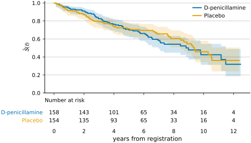
)

The two curves stay inside each other’s confidence bands. At five and ten years:

for label, code in [("D-penicillamine", 1), ("Placebo", 2)]:
    mask = arm_raw == code
    S_arm = ts.nonparametric.kaplan_meier(Y[mask], delta[mask])
    print(
        f"{label:18s}  5-year: {float(S_arm(5.0)):.1%}   "
        f"10-year: {float(S_arm(10.0)):.1%}   "
        f"(n = {int(mask.sum())}, events = {int(delta[mask].sum())})"
    )

D-penicillamine     5-year: 70.8%   10-year: 42.5%   (n = 158, events = 65)
Placebo             5-year: 71.5%   10-year: 45.7%   (n = 154, events = 60)

The arms differ by less than one percentage point at five years and by 3.2 points at ten, in line with the trial’s published conclusion that D-penicillamine showed no survival benefit. With 125 deaths, the absence of a visible difference does not show that the effect is zero; it limits how large the effect can plausibly be.

A covariate that does matter: histologic stage

Histologic stage is the pathologist’s reading of biopsy material at baseline, scored 1 (mild fibrosis) to 4 (cirrhosis). Unlike treatment, it was not randomised.

stage_raw = X["stage"].to_numpy()
has_stage = ~np.isnan(stage_raw)
stage = stage_raw[has_stage].astype(int)

ts.plot.km(
    Y[has_stage],
    delta[has_stage],
    group=np.array([f"stage {k}" for k in stage]),
    xlabel="years from registration",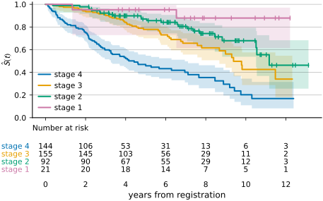
)

The four curves separate early and stay apart. At five and ten years:

for k in range(1, 5):
    mask = stage_raw == k
    S_k = ts.nonparametric.kaplan_meier(Y[mask], delta[mask])
    print(
        f"stage {k}  5-year: {float(S_k(5.0)):.1%}   "
        f"10-year: {float(S_k(10.0)):.1%}   "
        f"(n = {int(mask.sum())}, events = {int(delta[mask].sum())})"
    )

stage 1  5-year: 95.2%   10-year: 87.9%   (n = 21, events = 2)
stage 2  5-year: 87.0%   10-year: 67.9%   (n = 92, events = 23)
stage 3  5-year: 77.9%   10-year: 42.6%   (n = 155, events = 48)
stage 4  5-year: 46.9%   10-year: 20.2%   (n = 144, events = 84)

Ten-year survival falls from 88% in stage 1 to 20% in stage 4, and fewer than half of stage 4 patients are alive at five years. Stage 1 has only 21 patients and 2 deaths, so its curve is the least precise.

What Kaplan-Meier does and does not give you

Kaplan-Meier estimates the marginal survival of a population, split by at most one categorical covariate at a time. It does not give:

• The magnitude of an effect adjusted for other covariates. The stage effect above is unadjusted; some of the visible separation may be confounded by age or baseline lab values.
• A single-number summary of the contrast that you can put in a paper or a clinical-decision aid.
• How to predict survival for a new patient given their covariates.

Modeling risk with covariates fits a Cox proportional-hazards model to this cohort, adjusts for several covariates at once and summarises the stage effect as a hazard ratio.

References

• Therneau, T. & Grambsch, P. (2000). Modeling Survival Data: Extending the Cox Model. Springer. Describes the PBC data.
• Pocock, S. J., Clayton, T. C. & Altman, D. G. (2002). Survival plots of time-to-event outcomes in clinical trials: good practice and pitfalls. Lancet 359(9318), 1686-1689.